How To Add Color Animation In C++ Qt

Bar plot is pretty bones and very common. All the plotting libraries take bar plot options for sure. This article volition focus on the animated bar plot. I will share the code for some animated bar plots. If you haven't seen them before, you lot may bask them.

I tried to present them simply and then that it is understandable. I ever like to offset with the basic plots. Here I am starting with two plots that are inspired by this page.

I had to install 'ImageMagick' in my anaconda surroundings using this command below because I wanted to save those plots to upload here. Yous may want to save your blithe plots to upload or present somewhere besides.

          conda install -c conda-forge imagemagick

These are some necessary imports:

          import pandas as pd
import numpy as np
from matplotlib import pyplot as plt
import seaborn as sns
from matplotlib.animation import FuncAnimation

Here is the complete code for a basic blithe bar plot. I volition explicate the code after the lawmaking and the visualization part:

          %matplotlib qt
fig = plt.figure(figsize=(viii,6))
axes = fig.add_subplot(1,1,1)
axes.set_ylim(0, 120)
plt.mode.utilize("seaborn")
                    lst1=[i, two, iii, 4, 5, 6, seven, 8, 9, 10, 11, 12, thirteen, 14, 15 ]
lst2=[0, five, 10, 15, 20, 25, 30, 35, 40, 50, 60, 70, 80, ninety, 100]
                    def animate(i):
            y1=lst1[i]
            y2=lst2[i]plt.championship("Intro to Animated Bar Plot", fontsize = 14)
anim = FuncAnimation(fig, animate, frames = len(lst1)-1)
anim.salvage("bar1.gif", author="imagemagick")

Now let's come across how the code works. Showtime I created two lists for ii bars.

The animate function here takes the elements of two lists and creates two bars named 'one' and '2' using 2 lists y1 and y2.

The FuncAnimation role actually creates the blitheness. It takes the animate function and the length of the data.

To salve the plot, nosotros need to provide a proper name for the plot. Here I used a very ordinary name, 'bar1.gif'. It uses 'imagemagick' we installed in the beginning to write the plot.

This one is almost the same as the first one with more than bars hither.

          %matplotlib qt
fig = plt.effigy(figsize=(eight,6))
plt.mode.apply("seaborn")
axes = fig.add_subplot(ane,i,ane)
axes.set_ylim(0, 100)
                    l1=[i if i<twenty else 20 for i in range(100)]
l2=[i if i<85 else 85 for i in range(100)]
l3=[i if i<xxx else 30 for i in range(100)]
l4=[i if i<65 else 65 for i in range(100)]
                    palette = listing(reversed(sns.color_palette("seismic", 4).as_hex()))
                    y1, y2, y3, y4 = [], [], [], []
def animate(i):
            y1=l1[i]
            y2=l2[i]
            y3=l3[i]
            y4=l4[i]plt.bar(["ane", "two", "iii", "four"], sorted([y1, y2, y3, y4]), color=palette)
            plt.championship("Blithe Bars", color=("blue"))
anim = FuncAnimation(fig, animate, frames = len(l1)-1, interval = 1)
anim.salve("bar2.gif", writer="imagemagick")

Notice here I included axes.set_ylim in the beginning. If you do not set the y-limit, the plot will animate like this:

I saw an blithe bar plot that went viral on social media on Covid'southward death a few months ago and decided to bank check how to exercise information technology. Here I am sharing that plot.

For the side by side plots, I will use this superstore dataset. Please feel free to download the dataset from hither.

The writer mentioned in the description of the page that it is allowed to use this dataset for educational purposes only.

Let's import the dataset and await at the columns:

          df = pd.read_csv("Superstore.csv", encoding='cp1252')
df.columns

Output:

          Index(['Row ID', 'Club ID', 'Lodge Date', 'Ship Appointment', 'Ship Mode',
            'Customer ID', 'Customer Name', 'Segment', 'Country', 'City', 'State', 'Postal Code', 'Region', 'Product ID', 'Category', 'Sub-Category', 'Production Name', 'Sales', 'Quantity', 'Discount', 'Turn a profit'], dtype='object')

Equally you can come across the dataset is pretty big. Just nosotros will merely use the 'Social club Date', 'Profit', and 'Land' columns for the adjacent plots.

The plots will exist on monthly total sales per state.

Nosotros need to perform some information preparation for this. Because we volition use bar_chart_race function for this and this part needs a sure format of data for the plot.

First thing is, that the 'Order Date' cavalcade needs to be in 'datetime' format.

          df['Guild Date'] = pd.to_datetime(df['Club Date'])

I will use pivot_table role to have each country's Sales information as the cavalcade:

          pv = df.pivot_table("Sales", index = "Order Date", columns = ["State"], aggfunc = np.sum)

Hither is the part of the output:

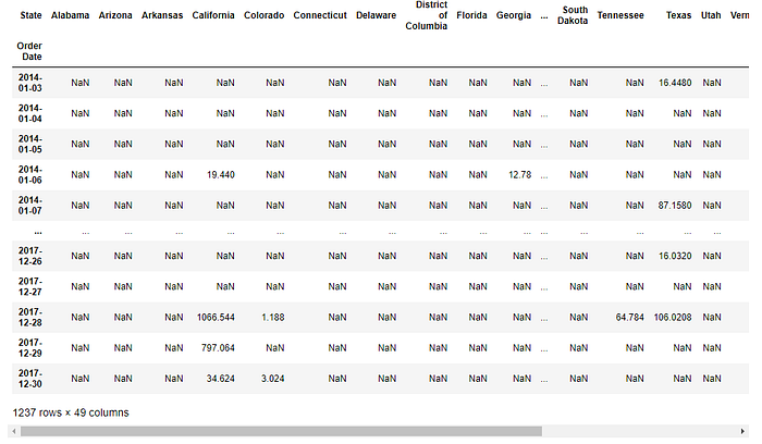
It gives the states so many null values because Sales data for each day is not available. Notice that the 'Order Appointment' column is the index now.

I will fill those zip values with zeros. Likewise, I am sorting the dataset by 'Lodge Date'

          pv.sort_index(inplace=True, ascending=True)
pv = pv.fillna(0)

Now, nosotros take all the nada values replaced past zeroes.

As I mentioned before, I want to meet the Sales per state by month. So, I will omit the date part and keep the calendar month and year role from the 'Social club Engagement' just.

          pv['month_year'] = pv.index.strftime('%Y-%thou')
pv_month = pv.set_index("month_year")

You volition see the dataset a bit later on.

If we want to get the monthly data, we take to use group by on the month_year data.

          pv_month.reset_index()
pv_monthgr = pv_month.groupby('month_year').sum()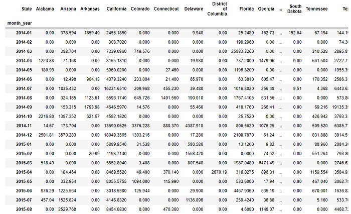

This is what the dataset looks like now. Nosotros take the monthly Sales data per state. Information technology is required to have the dataset in this format to utilise the bar_chart_race function.

I should warn you that it takes a lot longer to render these plots than regular bar plots. Sometimes it got stuck when I was doing them for this tutorial. I had given a little break to my reckoner and come dorsum afterward to restart my kernel then it worked faster. But notwithstanding, it takes longer overall.

Here is the bones bar_chart_race plot.I am using filter cavalcade colors parameters equally True and so that it does not repeat the colors for bars.

          import bar_chart_race as bcr
                    bcr.bar_chart_race(df = pv_monthgr,            
filename = "by_month.gif",            
filter_column_colors = True,            
cmap = "prism",            
title = "Sales Past Months")

Y'all can see that it is sorted in descending order by default. Every month the order of united states of america changes. Only it is moving and then fast that it is hard to encounter the name of u.s. even. In the bottom correct corner, it shows the month.

In the next plot, we will run into some improvements. period_length parameter controls the speed. I used 2500, which is pretty loftier. Then, it will show i month a lot longer than the default.

At that place is n_bars parameter to specify how many bars we desire to see in 1 frame. I am fixing it at 10. Then nosotros volition run across the superlative ten states based on sales amount for every month. The 'fixed_max' parameter will fix the x-centrality to the overall maximum Sales value. And so it will not change in every frame.

          bcr.bar_chart_race(df=pv_monthgr,
filename="bar_race3.gif",            
filter_column_colors=True,            
cmap='prism', sort = 'desc',            
n_bars = 10, fixed_max = True,            
period_length = 2500,            
title='Sales Past Months', figsize=(10, 6)))

In the next plot, We volition add together 1 more piece of information in the plot. Each frame is showing the plot for a month. In the bottom right corner, it will testify the total sales amount of that month.

For that, I added a function called summary. I also included some more style parameters.Bar label size, bar-mode that makes it a scrap transparent and gives a border. Nosotros are also adding a perpendicular bar that volition show the mean sales for each month. Each month the mean sales vary. So, the perpendicular bar will keep moving.

          def summary(values, ranks):
            total_sales = int(circular(values.sum(), -2))
            s = f'Full Sales - {total_sales:,.0f}'
            return {'x': .99, 'y': .1, 's': s, 'ha': 'right', 'size': 8}          bcr.bar_chart_race(df=pv_monthgr,filename="bar_race4.gif", filter_column_colors=True,
            cmap='prism', sort = 'desc', n_bars = 15,
            fixed_max = True, steps_per_period=3, period_length = 1500,
            bar_size = 0.8,
            period_label={'10': .99, 'y':.xv, 'ha': 'correct', 'colour': 'coral'},
            bar_label_size = 6, tick_label_size = ten,
            bar_kwargs={'blastoff':0.iv, 'ec': 'black', 'lw': 2.5},
            championship='Sales Past Months',
            period_summary_func=summary,
            perpendicular_bar_func='mean',
            figsize=(7, 5)
            )

This volition exist the terminal plot where I will add 1 more function that will add a custom role to add the 90th quantile in the bar. The steps_per_period equal to three means, it takes three steps to get to the next frame. If you notice by the fourth dimension a month changes in the bottom right corner label, the bars moved three times and y'all can see how they overlap and slowly change their position.

          def func(values, ranks):
            return values.quantile(0.9)          bcr.bar_chart_race(df=pv_monthgr,filename="bar_race5.gif", filter_column_colors=True,
            cmap='prism', sort = 'desc', n_bars = 15,
            steps_per_period=3, period_length = 2000,
            bar_size = 0.8,
            period_label={'x': .99, 'y':.15, 'ha': 'right', 'color': 'coral'},
            bar_label_size = 6, tick_label_size = ten,
            bar_kwargs={'alpha':0.four, 'ec': 'black', 'lw': 2.v},
            title='Sales Past Months',
            period_summary_func=summary,
            perpendicular_bar_func=func,
            figsize=(7, 5)
            )

If you like vertical bars instead of horizontal ones, delight use orientation='v'. I prefer horizontal confined.

To learn more about all the unlike parameters y'all can use to change the plot, please visit this link.

Please experience gratuitous to try out some more mode options or different functions for the summary or the perpendicular bar.

You may also want to endeavor different colors, fonts, font sizes for labels and ticks

Conclusion

Though some people may argue that a simple bar plot shows the information more conspicuously. I concord with that besides. But still, it is proficient to accept some interesting plots like this in the collection. As you tin meet how each calendar month the ranking of us is changing as per the sales data, and how the mean sales or 90th quantile is moving. You cannot go a feel of this blazon of modify using a still plot. Also, if you have some interesting-looking plots, it grabs attention.

Please experience complimentary to follow me onTwitter, and theFacebook folio, and check out myYouTube aqueduct.

#DataVisualization #DataScience #DataAnalytics

#Python #Matplotlib #barplot

Source: https://regenerativetoday.com/animated-and-racing-bar-plots-tutorial/

Posted by: williamsannot1974.blogspot.com